General Linear Models
A general linear model describes a dependent variable in terms of a linear combination of independent variables and an error term.
Simple Linear Regression
A line can be described by the equation \(y = mx + b\), where \(b\) is the \(y\)-intercept and \(m\) is the slope. Simple linear regression uses this idea to describe the relationship between two variables—one dependent, the \(y\), and one independent, the \(x\). Dependent variables are also sometimes referred to as "response variables," "regressands," or "targets." The corresponding terms for independent variables are "predictor variables," "regressors," or "features."
The objective is to specify a model that explains \(y\) in terms of \(x\) in the population of interest. A simple model can be specified as follows.
\[y = \beta_0 + \beta_1 x + \epsilon\]
In this specification—called the scalar form—\(\beta_0\) represents the \(y\)-intercept and \(\beta_1\) represents the slope. The \(\epsilon\), which is called the error term, represents other factors that affect \(y\). If the error term is excluded, the implication is that the relationship is exact or deterministic. On the other hand, if we include the error term, we imply that the relationship also contains a stochastic component. For most, if not all, applications of regression, the relationship between the dependent and independent variables includes both deterministic and stochastic parts.
The actual \(\beta\) values in the population are unknown. However, they can be estimated using data—preferably a random sample from the population. We use this data to find the line that "best" fits it. Because each observation in our sample has its own values, we use subscripts to denote them.
\[y_i = \beta_0 + \beta_1 x_i + \epsilon_i\]
Notice that the \(y\), \(x\), and \(\epsilon\) terms have subscripts, but the \(\beta\)s do not. This implies that there is a single \(y\)-intercept and slope—the one from the population equation that represents the "true" line.
Multiple Regression
Often, outcomes for our variable of interest, \(y\), depend on two or more predictors. This is referred to as a multiple linear regression model, which, for the case of two variables, can be written as:
\[y_i = \beta_0 + \beta_1 x_{1i} + \beta_2 x_{2i} + \epsilon_i\]
As you might imagine, the scalar form gets unwieldy as the number of independent variables increases. To deal with this, we introduce an alternative way to express our model.
Matrix Form
While the scalar form allows us to be explicit about the regressors included in the model, it is often more efficient to write the equation in matrix form. To motivate the reasons why, consider the case where, for our equation above, \(i = 1, 2, \ldots,n\).
\[y_1 = \beta_0 + \beta_1 x_{11} + \beta_2 x_{21} + \epsilon_1\] \[y_2 = \beta_0 + \beta_1 x_{12} + \beta_2 x_{22} + \epsilon_2\] \[\vdots\] \[y_n = \beta_0 + \beta_1 x_{1n} + \beta_2 x_{2n} + \epsilon_n\]
Our system of \(n\) equations can, instead, be represented in terms of matrix addition. Note that we've included a vector of ones of length \(n\), which we'll call \(x_0\), that we multiply with \(\beta_0\).
\begin{split} \left[\begin{matrix}y_1\\ \vdots\\ y_n\end{matrix}\right] = \beta_0 \left[\begin{matrix}1 \\ \vdots\\ 1\end{matrix}\right] + \beta_1 \left[\begin{matrix}x_{11}\\ \vdots\\ x_{1n}\end{matrix}\right] + \beta_2 \left[\begin{matrix}x_{21}\\ \vdots\\ x_{2n}\end{matrix}\right] + \left[\begin{matrix}\epsilon_1\\ \vdots\\ \epsilon_n\end{matrix}\right] \end{split}
This can be restated in terms of matrix multiplication.
\begin{split} \left[\begin{matrix}y_1\\ \vdots\\ y_n\end{matrix}\right] = \left[ \begin{matrix} 1 & x_{11} & x_{21}\\ \vdots & \vdots & \vdots\\ 1 & x_{1n} & x_{2n} \end{matrix} \right] \left[\begin{matrix}\beta_0\\ \beta_1\\ \beta_2\end{matrix}\right] + \left[\begin{matrix}\epsilon_1\\ \vdots\\ \epsilon_n\end{matrix}\right] \end{split}
Here, we've simply combined the \(x_0\), \(x_1\), and \(x_2\) into a matrix, which we refer to as \(X\), called the design matrix, and combined the \(\beta\)s into a column vector, which we refer to as \(\vec{\beta}\), called the parameter vector. In this example, \(X\) is an \(n \times p\) matrix and the column vector \(\vec{\beta}\) can be thought of as a \(p \times 1\) matrix, where \(p = 3\). Because the number of columns in \(X\) equals the number of rows in \(\vec{\beta}\), they can be multiplied, resulting in an \(n \times 1\) column vector. This is the deterministic portion of our model, which, when added to the stochastic component, \(\vec{\epsilon}\), results in \(\vec{y}\).
The matrix form of our model can be rewritten compactly using vector notation.
\[\vec{y} = X\vec{\beta} + \vec{\epsilon}\]
This specification can handle an arbitrary number of parameters. For each parameter, \(p\), add a column to \(X\) and an element to \(\vec{\beta}\).Solving
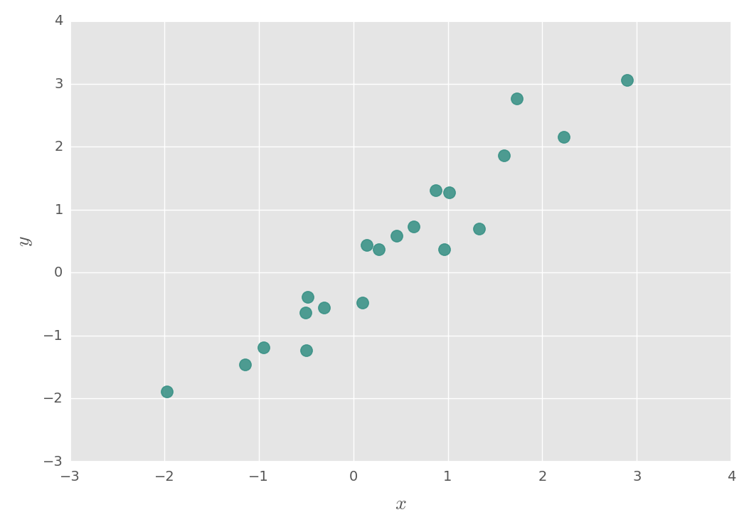
There are several ways to solve for the "best" line. To illustrate this, we'll go back to the simple linear regression model. Let's suppose we'd like to create a regression line for the data shown in the following plot, created using the code below. (Note: the complete set of commands used to make this plot can be found here.)
import numpy as np
import matplotlib.pyplot as plt

np.random.seed(1868)
x = np.random.normal(0, 1, 20)
y = np.array([np.random.normal(v, 0.5) for v in x])

plt.scatter(x, y, s=35, alpha=0.85, color='#328E82')
The "best" line is usually thought of as the one that minimizes the vertical distance between it and the data points. Typically, the distance that is minimized is the sum of the squared residuals. This is the ordinary least squares estimation. Residuals are the difference between each \(y_i\) and its estimated (or fitted) value, \(\hat{y}_i\). In vector notation, these can be written as \(\vec{y}\) and \(\hat{\vec{y}}\), respectively. The idea is to find values of \(\beta_0\) and \(\beta_1\) that minimize: \[\sum_{i=1}^n (y_i - \hat{y}_i)^2\]
The terms "errors" and "residuals" are often used as synonyms, unfortunately. In reality, they are quite distinct. Errors are a population-level concept and are unobservable. Residuals, on the other hand, are sample-specific and are computed from the data when we estimate the \(\beta\)s.
Recall that we can specify the model for the data above as \(\vec{y} = X\vec{\beta} + \vec{\epsilon}\). From this, we can use matrix algebra to estimate the "best" line.
\[\hat{\vec{\beta}} = (X^T X)^{-1} X^T \vec{y}\]
Using NumPy, we can estimate the parameter vector as follows.
import numpy.linalg as npl

ones = np.ones(len(x))
X = np.column_stack((ones, x))
b = npl.inv(X.T.dot(X)).dot(X.T).dot(y)
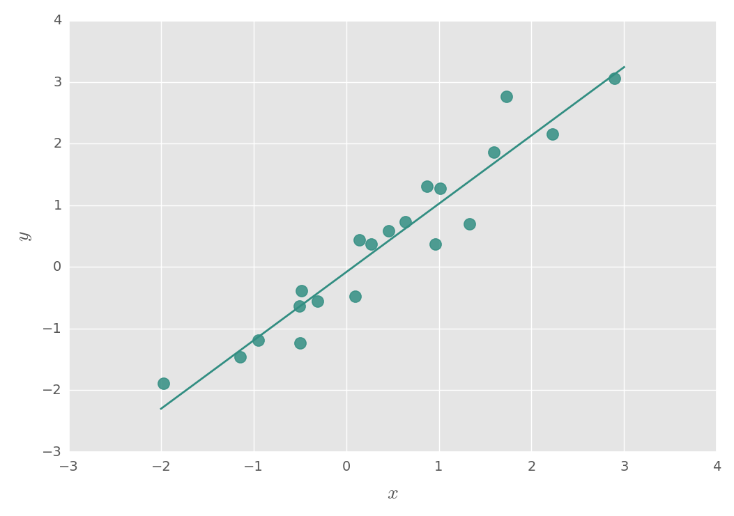
Here, \(b\) is the estimated \(\hat{\vec{\beta}}\) with values [-0.08396926, 1.10769145]. These represent \(\hat{\beta}_0\) and \(\hat{\beta}_1\), respectively. This results in the following regression line, in which is the sum of the squared distances between the data points and the line have been minimized.
For this approach to work, \(X^T X\) must be invertible or nonsingular. This means that the columns in \(X\) must be linearly independent. If this isn't the case—that is, if \(X^T X\) is not invertible—then there will be an infinite number of solutions for \(\hat{\vec{\beta}}\).
The General Linear Model
"The term general linear model refers to a linear model of form \(\vec{y} = X\vec{\beta} + \vec{\epsilon}\)" (Poline and Brett). It's "general" in the sense that the data in \(X\) can be continuous, discrete, or even binary (dummy). The errors, \(\vec{\epsilon}\), are assumed to be independent and identically distributed with a zero mean and \(\sigma^2\) variance. General linear models need not only describe a single \(y\). That is, they can also cover multivariate models.
Final Thoughts
We've seen how to construct simple and multiple linear regression models using matrix notation and how to estimate the parameters using NumPy. These models are useful and are used often for describing the relationships between variables.
The following sources were invaluable for my
understanding of these concepts.